Chapter 1: Introduction
Read carefully – a short test will follow the text of the intro.
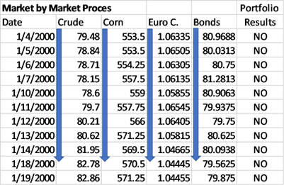
I have created my own little universe and I call it TradingSimula-18. If you want to learn python and algorithmic end of day trading, then come along this journey with me. I love TS-18 because it only relies on one external library, and it does exactly what you need it to do. It is mostly open source, so you can get in there and bugger it up or make it better or change it. It comes with its own small database, but you can easily change that. It is compatible with any ASCII format if you have the minimum of a date, open, high, low and close fields. It can accept volume and open interest as well. The database is quite simple – you have one dataMaster.txt file and one file for each individual market (continuous linked format.) I use PyScripter as my go to IDE, but you can use any you like. I have used Sublime and IDLE, and they work great. TS-18 could have a much simpler interface if it didn’t span the portfolio horizontally. TradeStation tests markets individually and sequentially, whereas TS-18 tests all markets combined in a sequential manner. Let us say you have a three-market portfolio of bonds, crude, and beans. Visualize it like a large table where the first column is the date, and the following columns are the closing price of each market. Each row has a specific date that relates to all the closing prices for each market in the table – like a simple spreadsheet. TS-18 first looks at the current day of the bond market and does all its calculations to determine trade entry/exit. Remember up to this date, TS-18 has access to all the current test market data. On the same day, it looks at crude and then beans. It hops from one market from the left to the right. By the time it reaches the last column, it knows all the information it needs to make a trading decision for the next trading day. Akin to a portfolio manager. Now, imagine that the rows not only contain the closing price for each market, but all the open, high, low prices too! Now our two-dimensional spreadsheet starts to look like a cube. For this reason, variables are handled a little differently in TS-18 by providing three primitive data types:
Variable Types
Scalar – flat dimension. This type of variable is recalculated each day for each market in the portfolio.
List – two dimensions. This type of variable is stored for each market in the portfolio as it is not recalculated on each day for each market in the portfolio.
List of Lists – three dimensional. A list with a memory.
This is the hardest concept to grasp for newcomers to TS-18
In EasyLanguage all variables are bar arrays meaning that they have history associated with them. When you define a variable in EasyLanguage:
vars: myVar(0);
You can query the prior values of myVar like this myVar[1] or myVar[2]. This is easy for TradeStation, because it does not hop from one market to another. Since we hop from market to market in a single portfolio day - the type of variable that you use depends on when it is calculated and if it needs to have a memory. The python list is very powerful and it acts very similar to an array. But it is even better because you have different methods like sort, delete, append and other functions that you can apply to your lists. Here is an example of using lists in python:
>>> mylist = list() #creates an empty list >>> mylist.append('apple') #adds the string ‘apple’ to the list >>> mylist.append(42) #adds the number 42 to the list >>> clist = ([1,2,3,4]) #create a new list clist and add a sub list >>> mylist.append(clist) #add the sub list to mylist>>> mylist #show me the list ['apple', 42, [1, 2, 3, 4]]If you need to access the individual elements of a list that is contained in another list, you can access it using the following format listname[2][0]
xxxxxxxxxxmylist[2][0] = 1 #lists are zero based -look at 3rd element (a list) and extracts 1st element of the list sub listmylist[2][3] = 4 #looks at 3rd element and extracts 4th element of sublistAs you can see lists in python are mutable - they can contain different data types - strings, integers, floats all in the same list. They can even be a list of lists. The last element in mylist is clist which is a list. Look at these variable names.
xxxxxxxxxx#variables section-----------------------------------------------------–#simple or scalar variableslongExit = 0 shortExit = 0profitLevel = 0liqLevel = 0If you need to create a simple list that remembers a value from one market to the next you can use the markettVal function.
curMarketRisk = marketVal(numMarkets) #list of 1 value for each market
Why do I need to do this?
If you need to create a bar list - a list that remembers each a variable’s history for each market, then you can use the barList function. This function requires the number of markets and the number of values to initialize and what those values are initialized to. The following code creates a list of lists named lagBarList with 5 elements in each list that are all zeros.
#list of lists - stores entire history of variable
lagBarList = barList(numMarkets,5,0)
Example usage of the three data types
Scalar or flat dimension
The following variables are calculated on each bar of data for each market. All you need to do is assign the variable name to some default values. Just like you do in EasyLanguage. Here I will need these four variables later in the program. Here is an example of using the simple variable:
longExit =  shortExit = profitLevel = liqLevel = 0
shortExit = highest(h, 20, D, 1)
These variables do not need to have a memory because they are renewed or recalculated on each daily bar for each market.
One dimension or market variable
These variables are not calculated on each bar so they need to be stored from one hop to the next. Assign your variable name (a list and be as creative as possible) to the return of the function call. MarketVal is a function that creates a one dimensional like array list in python.curMarketRisk = marketVal(numMarkets)
or you can add the values you want to assign the list
buyLevels = marketVal(numMarkets,999999999)
buyLevels will be initialized with nine 9s.
If your portfolio contains three markets, then your variable name list will look like this.
xxxxxxxxxxcurMarketRisk[0] = 0 // might be British PoundcurMarketRisk[1] = 0 // might be EurocurMarketRisk[2] = 0 // might be bondsThis is an example of storing a single value from hop to hop. Why would you want to do this. Say you want to store the value of the trade risk only when a long or short position is initiated. The following code is going to initiate a long position at the next bars open. We know it is going to do this because the criteria is tested and if it passes, then a long position at the market will be initiated. Because we know a long position will be put on, we can store the tradeRisk in the curMarketRisk[curMarket] or curMarketRisk[cm] list (cm is a short cut for currentMarket).
xxxxxxxxxx if close[D1] > Donch_HI and close[D1] > Upper_Band and \ tradeRisk < Initial_Risk and not(long) : price = open[D] tradeName = "l-entry" curMarketRisk[curMarket] = tradeRisk tradeTicket.append([buy,tradeName,posSize,price,mkt])Don’t worry if you don’t fully understand what this code is doing. But, I bet you can glean some information from it. Here if the close of yesterday (D1) is greater than the Donchian high and the close of yesterday is greater than an upper band and the current trade risk is less than initial risk and we are not currently long then add a long position via a market (mkt) order to our trade ticket. But before we add the order, we store the days tradeRisk into our curMarketRisk[curMarket] variable name. It is so very important to use the square brackets and the curMarket or cm as an index. Again we do this because we are capturing a value that is just calculated occasionally. Yes, tradeRisk is calculated daily, but we only want to keep track of the value when a trade is initiated.
Three dimension or bar list variable
This sound really complicated, but it isn’t. This is just a list that jumps from one market to another. In other words the historic values of the variable will be at our finger tips.
numMarkets = 3
lagBarList = barList(numMarkets,5,0)
The above creates a list with the name lagBarList and fills it with three (numMarkets) lists. Initially all the three lists are filled with five zeros. lagBarList is a list of lists that stores the entire history of the Laguerre RSI calculation for each bar for each market. It could look like this.
lagBarList[0] = [0.87,0.83.0.84,0.64,1.0] // might be British Pound lagBarList[1] = [0.97,0.81.0.84,0.69,0.95] // might be Euro lagBarList[1] = [0.89,0.71.0.64,0.29,0.15] // might be bondsx lagBarList[cm].append(LagRSIList[cm].calcLaguerreRSI(myClose,0.5,D,1))
longEntry = lagBarList[cm][-1] < .2 and lagBarList[cm][-2] > .2 shortEntry = lagBarList[cm][-1] > .8 and lagBarList[cm][-2] < .8longEntry will either be True or False. If the last value of the current market's Laguerre RSI ( lagBarList[][cm][-1] is < 0.2 and the prior Laguerre RSI ( lagBarList[cm][-2]) is greater than 0.2, then you have a crossing below 0.2 from above and longEntry will be set to True. Remember the Bar List variables must contain which market [cm] and values must be APPENDED to each list. Once you append them, you can access their history.
Remember to always use curMarket or cm in the index of your non simple variable names.
List constructs provided to the user
Use the generic name or assign them to your own variable name. Here are the lists names that can be utilized. If you don't want to create your own variable names - the following are predefined.
Two dimension or market variable:
marketVal1
marketVal2
marketVal3
marketVal4
marketVal5
marketVal6
marketVal7
marketVal8
Usage: Assign value
Store values in these simple lists like this: marketVal1[curMarket] = 42
Three dimension or bar list variable:
marketVal1List
marketVal2List
marketVal3List
marketVal4List
marketVal5List
marketVal6List
marketVal7List
marketVal8List
marketVal9List
marketVal10List
marketVal11List
marketVal12List
Usage: Append value
Add or append elements to the marketVal*List using append: marketVal1[curMarket].append(42)
Two dimension or market variable of type Boolean
cond1
cond2
cond3
cond4
marketCond1
marketCond2
marketCond3
marketCond4
marketCond5
marketCond6
marketCond7
marketCond8
Usage: Assign True or False
marketCond1[cm] = True
cond1[cm] = False
End of Chapter Test
Question #1
I am calculating the Bollinger Bands for a strategy trading a multi-market portfolio. Do I have to declare/define anything ahead of time?
Answer #1
No. Since you are calculating these values of every bar of the data on every market so assign the function results to anything you want.
upper, lower, middle = BBands(close,80,2,D,1)
Question#2
I need to save the risk amount on the day I enter a trade. Do I have to declare/define anything ahead of time?
Answer #2
Yes. Since you are not recalculating this value on a daily basis, you need to store this value in a predefined marketVal1, marketVal2…marketVal10. Or create you own market value with the (marketValue()) function call.
Once you get a hang of the variables and their types you will be well on your way to testing very sophisticated algorithms.
Chapter 2: TradingSimula-18 Testing Paradigm and Installation
This is a very detailed explanation of the installation of everything you will need. If you already have Python, you can scan over a good portion of the text. You will need openpyxl so you will want to pay attention to this portion of the text.
TradingSimula-18 is the software I initially developed for my book, The Ultimate Algorithmic Trading System Toolbox + Website: Using Today's Technology To Help You Become A Better Trader. Written in Python, this powerful tool allows you to create your own trading algorithms. The software follows a similar approach to early back-testing systems, conducting market-by-market analysis. It fully processes the first market in the portfolio before moving on to the next, while simultaneously accumulating individual equity to be analyzed at the end of the test. As detailed in the introduction, this methodology was also employed by John Fisher in his development of Excalibur. Below is a schematic of the process:
This works okay if you don’t need to make daily portfolio decisions in the historic back test. If you want to adjust position size based on total daily portfolio equity, then you can’t do it. The newer version that was used in my later book (Pruitt, George. Trend Following Systems - 2nd Edition: A DIY Project: Batteries Included - Can you reboot yesterday's algorithms to work with today's markets?. George Pruitt, 2022.) employs the following process:
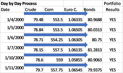
Here the looping mechanism runs through each market on a daily basis so at the end of each daily bar the total portfolio equity is known and can be used for the next bar’s action. You can also make other portfolio level decisions like limiting the total number of open positions; you may not want to be long bonds when you are already long notes. TradingSimula-18 works within a Python development environment so you must have Python already installed.
Installation of TradingSimula-18
TradingSimula-18 is a collection of python scripts, so all you need to do is unzip the zipped file to a folder to a convenient location on your computer.
TradingSimula_18 Starter Script
First time users to my TradingSimula_18 will want to go through this section. The following eight lines of code do a lot and if you can partially understand it at this stage you are definitely on your way:
xxxxxxxxxx01 buyLevel = highest(myHigh,80,curBar,1)02 shortLevel = lowest(myLow,80, curBar,1)03 longExit = lowest(myLow,20, curBar,1)04 shortExit = highest(myHigh,20, curBar,1)05 ATR = sAverage(myTrueRange,30, curBar,1)06 posSize = .005*dailyPortCombEqu/(ATR*myBPV)07 posSize = int(posSize)08 if posSize == 0 : posSize = 1Let’s start with line 01 – here a buy level is defined to be equal to the highest high 80 days back starting with a 1-bar offset. In other words, start with yesterday’s bar and work backwards for 80 days. myHigh (or high or h) is the list that contains all the high prices for the market being tested at the moment. TradingSimula-18 assumes you are sitting on the closing price of the current day in the back-test, and you can make a trading decision after the fact based off of today’s action. This is very powerful yet very dangerous. I allow future leak in this software. In other words, you can glimpse into the future to decide now. Many other testing platforms don’t allow for this, and it causes some limitations when backtesting. As long as you are aware of this capability and don’t abuse it, then you will be fine. The keyword (a word that is used internally and should not be altered by the user) highest is simply a function (a snippet of code that takes input and provides output) that returns the highest value going back x-days in history. In this case, it is returning the highest high going back 80 days. This function requires you to provide the following information as inputs: the data list (myHigh), the lookback time period (80), current bar (curBar), and offset (1). I got tired of typing curBar so I created the following variable names:
xxxxxxxxxx# Indexing into the daily bar dataD = curBar # high of today = high[D]D1 = curBar - 1 # high of yesterday = high[D1]D2 = curBar - 2 # high of day before yesterday = high[D2]...D10 = curBar - 10Using D1 is much better than using curBar - 1, right? Once this line is executed, the computer will find the function, pass the information to it, and then return the requested value – highest high for the past 80 days offset by 1. Lines 02 through 04 define the rest of the entry and exit levels. shortLevel is the price level that is defined to sell short. Notice the only difference between the code for the buyLevel and shortLevel is the name of the function – lowest versus highest. See how the same functions (as the entries) are used to set up the variables longExit and shortExit. The names used thus far (buyLevel, shortLevel, longExit, shortExit) are just holding places that contain certain values that will be used later in the program, or script if you like. These named storage are known as user-defined variables. In line 05 I create a new variable ATR and assign it the value of a 30-day moving average of myTrueRange. In this line of code, ATR represents the 30-day average true range. Unlike the prior functions that have been used, this function returns a non-price value. It only does this because I pass it a non-price data list, myTrueRanges. The function sAverage returns a simple moving average of whatever is sent to it via the data list. If I had used myClose in place of myTrueRanges, then the function would have returned a moving average of closing prices for the past 10 bars. Once I have calculated ATR I can move ahead and determine the position size for the next trade entry. Lines 6 through 8 handles this. Here a simple fixed fractional allocation method based off of perceived market risk (ATR) and the amount I am willing to risk on a per trade basis - 0.5% of total current portfolio equity is utilized.
If 0.5% of portfolio equity equates to $5000 and ATR equates to $2000 then position size (posSize) = 2.5 contracts ($5000/$2000). You can’t trade fractional contracts in the futures markets, so simply truncate the fractional part of the value (int(posSize)). The int function returns the whole part of the value that is passed to it. In some cases, the calculation for position size can wind up to be zero. I didn’t want this, so I set it to 1 in case the initial calculation ends up as zero. In some implementations of the fixed fractional allocation model, traders do allow a position size to take on the value of zero. In these scenarios the next trade is skipped because of its high volatility reading. This can be seen as a double-edged sword - the benefit is you skip an above average risky trade, and the drawback is you lose the trades contribution to the portfolio’s diversification. In eight lines of Python code, you defined your trading algorithm’s entry and exit levels and position size based on the daily snapshot of total portfolio equity. That’s quite a bit of work in just a few short lines of code.
Now that we have everything we need for a complete trading algorithm, let’s take that information and test it. Defining a trading system is just the first step, the next is actually putting it into some form of computer code. The code that you use to accomplish this task is highly dependent on the platform you are using to back-test. Python is the language of choice for the TradingSimula-18 platform so we will go that route. EasyLanguage translations for TradeStation and MultiChart users will also be included. Professional platforms try their best to eliminate the need for in-depth programming knowledge by their users. And they do a great job of that, but at a cost. These platforms try to use simple English like commands to effectuate a trader’s trading ideas. If the idea is simple, then there is no problem. If it’s a little more complicated, then the trader must dig deeper into the language and then the simple “English like” scripting language flies out the window. TradingSimula-18 does all the simulation and trading accounting for you, but you still need to know just a little of the real programming language, Python. In many languages, not C or Java, the syntax is at such a high level that it is very easy to learn without the need to create an “English-like” interface. Here is a snippet of the code that is used to actually put the algorithm to work in Python. The following logic is executing a stop order. Remember we are using the latest iteration of TS-18 with what I call “Trade Ticket Technology or TTT. I will show the old way of doing this, which can still be utilized and then the new way.
xxxxxxxxxx
buyLevel = RNT(buyLevel,up,minMove)
#TS-18 pre 2024 Editionif myHigh[curBar] >= buyLevel and mp !=1:    price = max(myOpen[curBar],buyLevel)    tradeName = "Simple Buy"    numShares = posSize    enterLongPosition(price,numShares,tradeName,sysMarkDict)    unPackDict(sysMarkDict)
#TS-18 – 2024 Editionif not(Long):    price = buyLevel    tradeName = “Simple Buy”    tradeTicket.append([buy,tradeName,posSize,price,stp])orif not(long):    tradeTicket.append([buy,”Simple Buy”,posSize,buyLevel,stp])
Pardon the interruption
Before going any further, I need to explain how you can access historical data during a back test. This is probably the most important thing when working with a new platform; it is the first thing I look for.
Accessing historic price action
TS-18 has different variables to access prior data. You can use them all or pick which one you prefer. Remember in most IDE, the variables, reserved and keywords are case sensitive.
Yesterday’s high
Examples of using curBar and D nomenclature.
xxxxxxxxxxmyHigh[curBar-1]high[curBar-1]h[curBar-1]myHigh[D1]high[D1]h[D1]
Day before yesterday’s high
xxxxxxxxxxmyHigh[curBar-2]high[curBar-2]h[curBar-2]myHigh[D2]high[D2]h[D2]
See the pattern?
xxxxxxxxxxD1 = curBar-1D2 = curBar-2D3 = curBar-3D4 = curBar-4
Data lists:
xxxxxxxxxxhigh, myHigh, hlow, myLow, lclose, myClose, cop, myOpen, o #note you can't use the word open - it is reserved**volume, myVolumemyOpenInt
Programming with/without Trade Ticket Technology
Prior to the 2024 edition, you had to test the high of today to see if it exceeded the buyLevel and if so then you knew the order would have been executed. This seems a little inconvenient, but it allows you to know if an order was 100% filled and you then could initiate logic based on this fact. You don’t need to do this in the 2024 edition, but you can if you like. In 2024, i prefer the multiple line order specification. It keeps you from having to cram everything into one line. Keep in mind there are times when you want to use the original method of order placement. For this reason I kept it backward compatible. The “trade ticket” technology or TTT allows you to place multiple orders during the trading day. All the information is fed into the TTT engine and the orders that should execute, will. The original method was top down programming, orders were initiated whenever the first of the entry/exit logic criteria was met. Because of this you had to use comparison logic to see which would have hit first. Assume you are long and you can reverse or get stopped out. TTT will pick just the order that would be elected first based on trade price and the current market price. Trend following systems usually only place a single order on a daily basis, so this did not hamper the original edition. The following code will get us out of a long position on a stop order.
xxxxxxxxxx#TS-18 pre 2024 EditionlongExit = RNT(longExit,down,minMove)if mp ==1 and myLow[curBar] <= longExit and barsSinceEntry > 1:    price = min(myOpen[curBar],longExit)    tradeName = "Lxit"    numShares = curShares    exitPosition(price,numShares,tradeName,sysMarkDict)    unPackDict(sysMarkDict)
#Current editionif long and barsSinceEntry > 1:    price = longExit    tradeName = "Lxit”    tradeTicket.append([exitLong,tradeName,curShares,price,stp])
What do you think? I want to go over the pre 2024 edition code first to help explain the trade ticket technology. You might not know the exact syntax, but you can surely get the gist of what is happening here. Starting with the first line in the first segment of code here is how it translates into English. If the high of the day is greater than or equal to buyLevel and mp (current market position) is not equal to one, then do something. Remember myHigh is a list of all the high prices in the data stream and curBar is an index into that list that represents the current bar in the back-test loop. If testing starts on June 1st, 2000, and that is the first bar in the data, then curBar would be equal to 1. Since I am not pyramiding I don’t want to add another long position, so I test for that. mp represents the current market position and here I am looking to see if it’s not equal to 1. In Python not equal is represented by != and equal is represented by ==. The test condition is then followed by the colon : If both conditions are true, then the flow of the program goes to the next line that is indented by four (4) spaces – remember the importance of indentation. If either of the conditions are false, the entire block of code that is indented is skipped. Let’s assume the current bar’s high price is greater than buyLevel. Consequently, the program flows to the next indented line of code that assigns price to the maximum of the open of the current bar or the buyLevel. Let’s stop here and comprehend what we are asking the computer to do. I am asking the computer if the extreme high price of the market exceeded the buyLevel, and if so, set the entry price to whichever value is larger: open of the bar or the buyLevel. In this example, the buyLevel is used as the stop price. Remember stop prices are above the market and are only elected once price breaches or reaches the stop order’s price. If the market open price gaps above the stop price, then price is set to the opening price of the bar. In earlier version of TradingSimula-18 I required this test for various reasons, and I will discuss this a little later. After the entry price is set, the tradeName is then assigned the value “Simple Buy” and lastly the numShares is set to the number of contracts calculated earlier with the fixed fractional scheme. Another chore you must attend to is making sure the price that you use for trade entry/exit is actually a price.
Without TTT: Rounding to the nearest tick increment
If you don’t use Trade Ticket Technology, then you must round the price to the nearest minimum move of the underlying market. Bonds and notes click in 32nds and 64ths:
130 1/32 = 130.03125
130 2/32 = 130.06250
130 3/32 = 130.09375
If your calculated entry price is 130.042456, you can still see if the price was elected by comparing it to the high of the day (STOP order), but this is not a valid entry price. TS-18 (before Trade Ticket Technology) will allow you to enter at 130.042456, but this price is actually between ticks (130 1/32 and 130 2/32.) You must round the price to a tick that existed. You have two options:
entryLevel = RNT(entryLevel,up,minMove)– this will move 130.042456 up to the next nearest tick, which is 130.0625 or 130 2/32. This makes sense since the market must tick to 130 2/32 to exceed 130.042456 and this is the tick you would be filled on. If the trade price falls exactly on a tick, then the price is left alone.entryLevel = RNT(entryLevel,0,minMove)– this will move 130.042456 to the nearest tick using rounding. Since 130.042456 is closer to 130.03125 than 130.0625, the price takes on the 130.03125 or 130 1/32 value. Again if the price falls right square on a tick value, then nothing happens.
The use of up or down or 0 depends on what you are trying to do:
Buy stop – entryLevel = RNT(entryLevel,up,minMove) – you are trying to buy above the market
Buy limit – entryLevel = RNT(entryLevel,down,minMove) – you are trying to buy below the market
Sell Short stop – entryLevel = RNT(entryLevel,down,minMove) – you are trying to sell short below the market
Sell Short limit – entryLevel = RNT(entryLevel,up,minMove) – you are trying to sell short above the market
When you exit a position you will either exit via a stop or limit or market order. Always round your entry level to a accurate tick using the RNT function. Market orders will execute at the open of the next day so you will not need to worry about this.
Once all the tasks are completed for the buy entry the indentation is removed.
With TTT: The computer rounds for you
I will now interject with the 2024 edition – you no longer need to test the high of the day against the buy level for a stop order. But you can if you so desire and in some cases you will want to use a combination of the test with TTT. And you no longer need to test if the open of the bar gapped through your stop order. TS-18 handles all this for you now. You can use mp == 1 or mp != 1 to determine current market position, but you can also use the keyword long or not(long). Next, in the second segment of code, the computer is being asked if the current position is long or 1 and the current bar’s low is less than or equal to the longExit price and barsSinceEntry is greater than 1. This code is testing to see if the long position that was put on via a stop in the first segment of code has been stopped out via the longExit stop. If all three conditions are met then the code that is indented is executed. That’s basically it! In EasyLanguage I could have done the same thing in just two lines of code (now with the 2024 edition you could do it with two lines as well.) Remember this is a very simple algorithm and like I mentioned earlier EasyLanguage and similar platforms make simple things simple to do. The flip side of the coin is basically the same, but with different price levels. Here is how to enter a short position and exit a short position on a stop basis.
xxxxxxxxxx#pre 2024 editionshortLevel = RNT(shortLevel,down,minMove)if myLow[curBar] <= shortLevel and mp !=-1:    price = min(myOpen[curBar],shortLevel)    tradeName = "Simple Sell"    numShares = posSize
shortExit = RNT(shortLevel,up,minMove)if mp ==-1 and myHigh[curBar] >= shortExit and barsSinceEntry > 1:    price = max(myOpen[curBar],shortExit)    tradeName = "Sxit"    numShares = curShares
#current editionif not(short):    price = shortLevel    tradeName = “Simple Sell”    tradeTicket.append([sellShort,tradeName,posSize,price,stp])if short:    price – shortExit    tradeName = “Sxit”    tradeTicket.append([shortExit,tradeName,curShares,price,stp])
#With the 2024 addition of Trade Ticket Technology, you no longer have to round the #trade level to fall exactly on a tick.  If the level is above the market, the price is #move up to the next tick and if the level is below the market, it is moved down to the #next tick.  If it falls exactly on a tick, then the price stays the same.
#At the top of the source listing, you will find the following code:
#-----------------------------------------------------------------------# Set up algo parameters here
#-----------------------------------------------------------------------startTestDate = 20000101 #must be in yyyymmddstopTestDate = 20051231 #must be in yyyymmddrampUp = 100 # need this minimum of bars to calculate indicatorssysName = 'DonchSimula2-1' #System Name hereinitCapital = 500000commission = 50
The pound sign or hash tag # lets the interpreter know that the text that follows is a comment and is to be ignored. Use this symbol when you want to explain what you are doing in the code. I use the symbol to provide comments where you need to get in the code that needs your attention. This section lets the user set the start and end test dates, the ramp up or the number of bars needed to properly calculate any indicators prior to the start test date, the system name, the initial capital, and commission amount charged for each round turn trade. You can add a slippage amount in dollars to the commission amount if you like.
You must decide on a database of EOD data
If you have just purchased TradingSimula-18 you get a small database of commodity futures data from Pinnacle Data and the database is already set up for you to dip your toe into how TS-18 works. I personally use Pinnacle Data, but CSI is great too! There are several companies that provide an updateable ascii database that can be used with TS-18. Any database in CSV format that includes at least date, open, high, low, and close fields, with a row for each date, can be utilized. Take a look at this code:
xxxxxxxxxx#--- Set Your Database Here ----------------------------------------------------#--- Make sure your dataMasterXXX.csv is set up properly with contract specs#--- Toggle comment to get your dataBase name - default is Pinnacle Data#-------------------------------------------------------------------------------dataBase = 'Pinnacle'#dataBase = 'CSI'#dataBase = 'Quandl'#dataBase = 'Custom'## R U using stock data? Set dataBase = 'Stocks'#dataBase = 'Stocks'## using first chars of fileName for symbol? if not set to 0useFirstNCharsAsSymbol = 2#----------------------------------------------------------------------------------
Right now you can use four databases:
Pinnacle - www.pinnacledata.org
CSI - www.csidata.com
Quandl - no longer updated, but their is history there
Custom - utilize your own or Norgate or some other data vendor
One of the more tedious things you must do before back testing futures data is to make sure your database dictionary is set up with the proper big point values and minimum price fluctuations. If you buy the CLDatabase from Pinnacle I have already set this up for you. If you use CSI data, and your output filenames use the first two letters to signify the symbol, then again I have already set this up for you. Using a back tester on futures data requires the data and a database dictionary (a dataMaster file). In TS-18 the dictionary is just a very simple csv file that contains four fields for each market. Here are the first few lines in the dataMasterPinnacle.csv file
xxxxxxxxxxAN_REV,1000,0.01,Aus.DolZL_REV,600,0.01,BeanOilBN_REV,625,0.01,B.PoundZU_REV,1000,0.01,CrudeZC_REV,50,0.25,CornCC_REV,10,1,CocoaCL_REV,1000,0.01,CrudeCN_REV,1000,0.01,Can.DolCT_REV,500,0.01,CottonFN_REV,1250,0.005,EuroCurDX_REV,1000,0.005,DolIndxED_REV,2500,0.0025,EuroDolEM_REV,100,0.1,MidCapMD_REV,100,0.1,MidCap
As you can see the variables are comma delimited. If you were to open this into a spreadsheet it would look something like this:
| File Name | BigPointValue | Min.Move | Market Name |
|---|---|---|---|
| AN_REV | 1000 | 0.01 | Aus.Dol |
| ZL_REV | 600 | 0.01 | BeanOil |
| BN_REV | 625 | 0.01 | B.Pound |
| ZU_REV | 1000 | 0.25 | Crude |
| ZC_REV | 50 | 1 | Corn |
| CC_REV | 10 | 0.01 | Cocoa |
| CL_REV | 1000 | 0.01 | Crude |
| CN_REV | 1000 | 0.01 | Can.Dol |
| CT_REV | 500 | 0.005 | Cotton |
| FN_REV | 1250 | 0.005 | EuroCur |
| DX_REV | 1000 | 0.0025 | DolIndx |
Most data vendors provide this information for you, and often you can obtain it directly from the CME, ICE, or other exchanges. However, when searching for this information, you might encounter an overwhelming amount of unnecessary data. Keep in mind that all you need to know are the file name, the big point value (BPV), and the minimum move.
Be aware that different data vendors may quote the market price using a different number of decimal places. This variation in quoted values will impact both the BPV and the minimum move. For example, CSI quotes a big point value of $125,000 and a minimum move of 0.00005 for the euro currency, while Pinnacle quotes the BPV as $1,250 and the minimum move as 0.005. Below are the euro currency quotes from the same day provided by these two vendors.
CSI Format
20240524, 1.08180000, 1.08610000, 1.08080000, 1.08500000
Pinnacle Format
05/24/2024,108.705,109.140,108.615,109.060,260776,654949
Don't be concerned about the absolute price differences, as both datasets have been smoothed to eliminate rollover gaps that occur at different times. Additionally, note that the CSI data does not include volume or open interest, which is perfectly fine if you’re using TS-18, as it only requires these four fields of data for historical backtesting. However, if your trading algorithm incorporates volume or open interest in its decision-making process, you will need to ensure that these fields are present in your data.
While all data vendors will provide consistent big point values (BPV) and minimum moves, the way they quote prices can vary. This variation often arises because the number of decimal places used in the quotes can differ. Essentially, vendors might scale the data by powers of ten, which can result in differences in how the BPV and minimum move are represented. For example, one vendor might quote a value with more decimal places than another, making it seem different, though they represent the same underlying market data.